|
Introduction Regression analysis deals with the relationship between one or more independent variables and a dependent variable. Regression analysis is performed by selecting a suitable function which accurately describes the relationship between the two and estimator to calculate the parameter values. These regression parameters are calculated by least squares method. In linear regression [1], either the parameters are linear or the function describing the model is linear. Nonlinear regression methods are applied when the relationship between dependent and independent variables in is not linear. Nonlinear regression relies on iterative procedure to find the best fit. The process [2] starts with initial values for each parameter, and then by using least squares fitting, the best fit parameter values which minimizes the sum of squared residuals are estimated. Microsoft Excel Solver Add-in estimates parameters for nonlinear regression by least squares method, but it doesn't estimate their precision. The paper aims to use finite difference method to estimate these values.
Nonlinear Regression A model is considered to be nonlinear if any of the partial derivatives with respect to any of the model parameters are dependent on any other model parameters, any of the derivatives do not exit or are discontinuous. A nonlinear model can be expressed as (equation 1):
where y is the vector of responses, f is the function used to describe the model, θ is vector of model parameters, t is the predictor variable and ε is the vector of residuals [3]. Rat43 dataset from National Institute of Standards and Technology (NIST) website [4], was selected to estimate the parameter precision by finite difference method. This dataset was selected, as the data can be fitted by using nonlinear regression method and is included in the higher level of difficulty group.
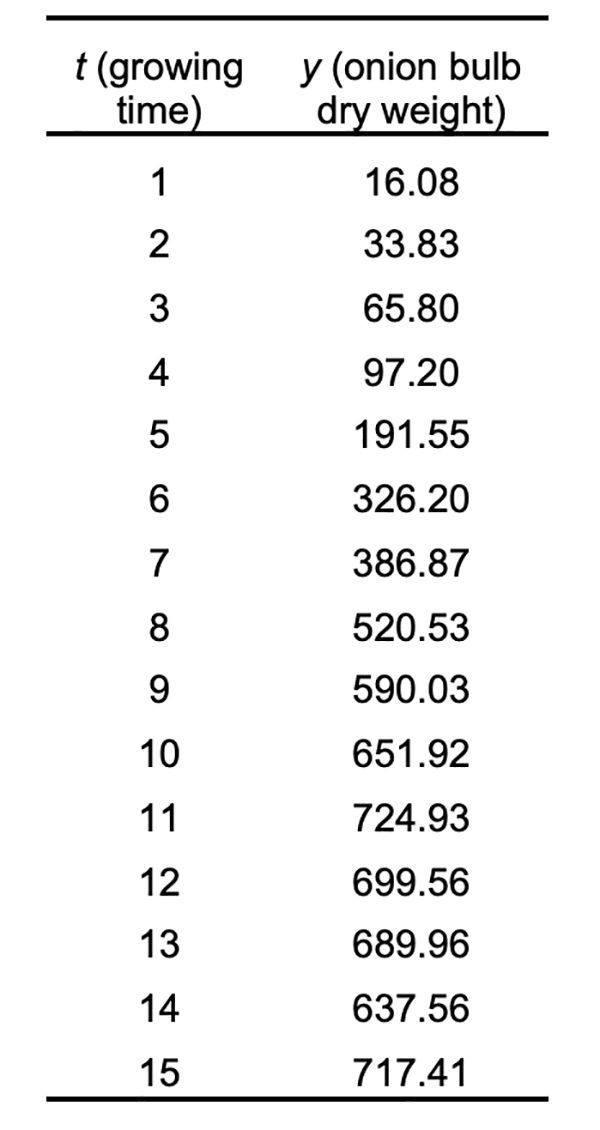
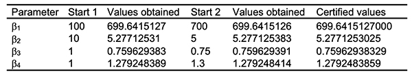
The nonlinear regression model described by equation 2 was used to fit the data, where response variable (y) is the dry weight of onion bulbs, whereas predictor variable (t) is growing time [4]. The model parameters were estimated by using both starting values and the results are given in Table 1.
Solver Implementation to Estimate Parameter Values (Table 2)
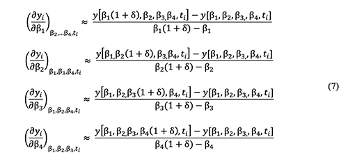
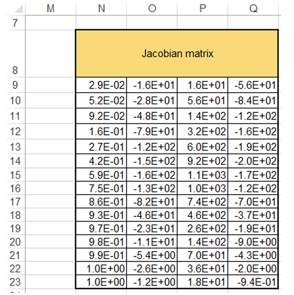
Finite Difference Method For a function with two or more independent variables, the partial derivative of that function with respect to a particular variable is the derivative of that function with respect to that variable, while holding the other variables constant [5]. The partial derivative term of each data point can by calculated by numerical differentiation. The parameter term (b1) is varied by a small amount from its optimized value while the other parameters terms are held constant. This variation of a parameter by a small amount is called perturbation. The partial derivatives are calculated by using the formula in Equation 7 [6] for all data points. Then the process is repeated for all the parameter terms in the model [6]. The Jacobian matrix (J) is constructed from all these partial derivative terms and is given by the following equation (3) [7], where m is the number of nonlinear parameters.
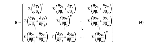
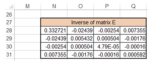
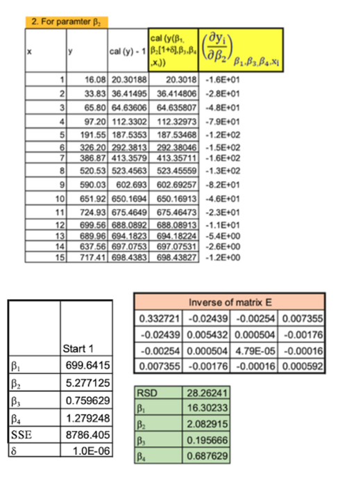
The parameter precision can be estimated from the matrix of partial derivatives (E), which is obtained by multiplying transpose of J with itself (E = JT * J) [7] and is given in equation 4.
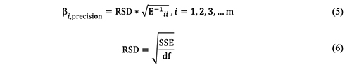
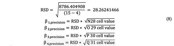
The square roots of the diagonal elements of was obtained from solver implementation the above E matrix inverse when multiplied and df is the degrees of freedom (difference by root residual standard deviation (RSD) between number of observation and number yields the precision for the respective parameter (equations 5 and 6) [7], where SSE value of parameters in the model).
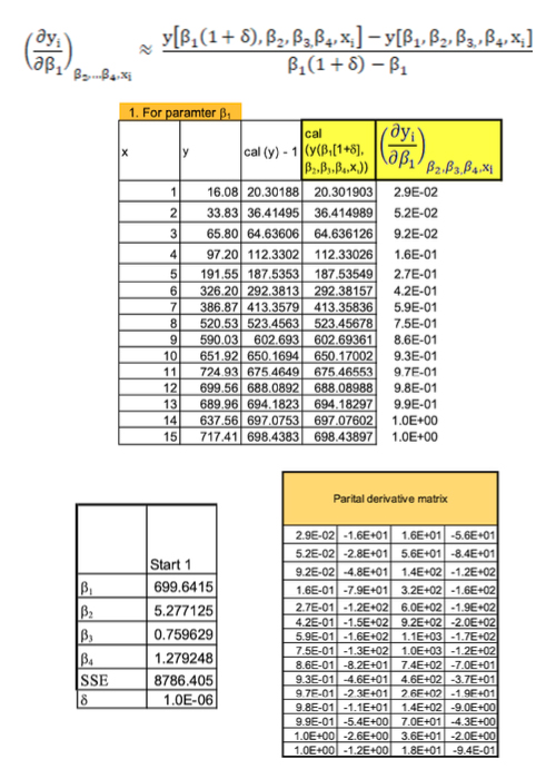
The individual partial derivatives for the J matrix can be calculated from the following equations (7) [7], where δ (perturbation) can be 10-6 or 10-7 [7]. The above calculations are performed in Microsoft Excel to obtain the parameter precision values for all the parameters.
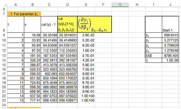
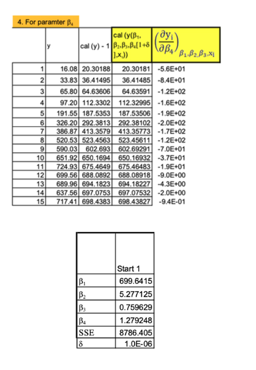
Results and Discussion The partial derivative calculations for the first parameter using parameter values obtained from Start 1 values are shown in Figure 1. Values in Column A9 to B23 corresponds to the raw data, values in C9 to C23 correspond to calculated values obtained after solver optimization. For values in D9 to D23, to the first parameter (β1) δ (10-6) was added and then its corresponding y (independent variable) values are calculated. The values in E9 to E23 are calculated as per equation 7. The calculations are repeated for all the parameters to obtain the partial derivative matrix (J), as given in equation 3.
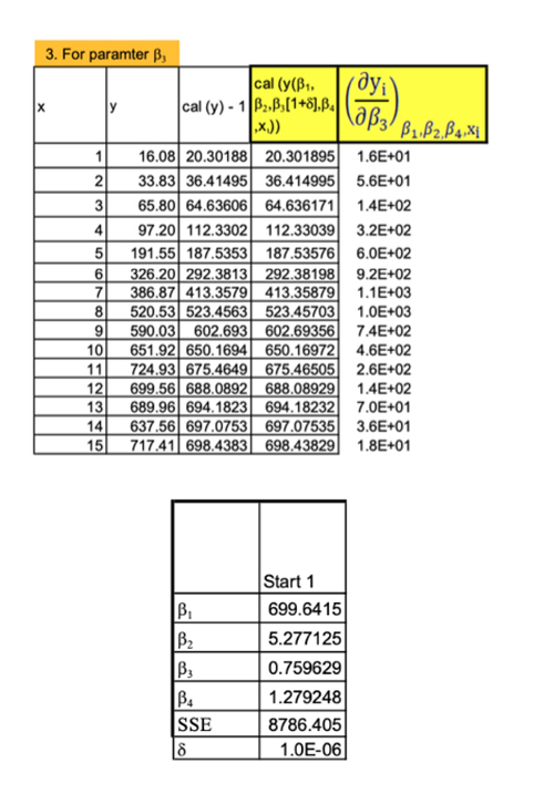
*** to view the complete Excel file, go to the appendix *** The Jacobian matrix in cells N9 to N23 are obtained by pasting the values of E9 to E23 for first parameter. The values O9 to Q23 in the matrix are obtained similarly from the other three parameters, and the resulting matrix is shown in Figure 2.
The result in Figure 3 is obtained by taking inverse of matrix E. The first parameter precision is obtained by multiplying the square root of value in N28 and RSD value (equation 8) [7].
Conclusions The parameter precision results obtained from the finite difference method were comparable to the reported values. Finite difference method offers a convenient approach to estimate nonlinear regression parameter precision values. Even though the method is robust in calculating precision values, limitations due to solver, like lack of convergence during optimization or parameter values inaccurately describing the model, can be encountered. For example, in the case of MGH10 dataset (which is available in the NIST website), the parameter values obtained after solver optimization are incorrect, which in turn leads to inaccurate parameter precision values.
References
|
||||||||||||||||||||||||||||||